

 English
 عربى
عربى
 Español


×
Password
Get password
Enter password to download relevant content.
Submit
 +86-15267462807
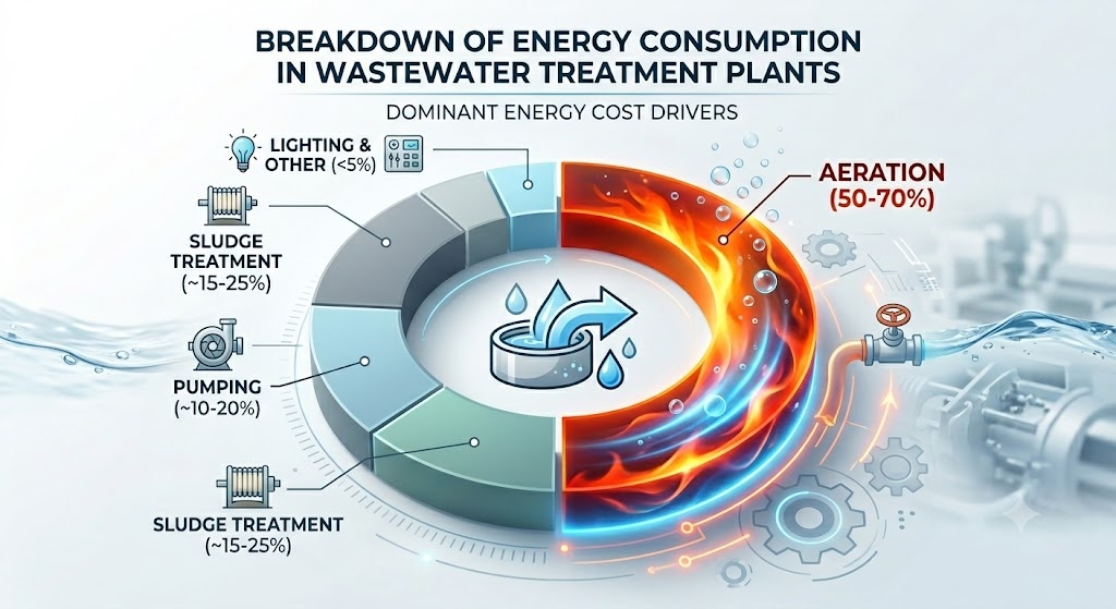
Direct answer: Aeration consumes 50–70% of total energy at a wastewater treatment plant. The core efficiency metric is Standard Aeration Efficiency (SAE), measured in kgO₂/kWh — how much oxygen your system delivers per unit of energy. A well-designed fine bubble diffuser system achieves 2.5–5.0 kgO₂/kWh. Most plants in operation fall short of this at 1.5–2.5 kgO₂/kWh due to fouled diffusers, oversized blowers running at part load, fixed DO setpoints that ignore diurnal load variation, and lack of VFD control. An energy audit identifies exactly which of these is costing the most — and the US EPA has documented that a properly designed aeration control system alone reduces aeration energy by 25–40%.
While aeration systems only account for 2–5% of construction costs, they consume up to 80% of the plant’s energy. Even at the conservative 50% figure, the numbers are substantial:
| Plant size | Typical total energy | Aeration share (60%) | At $0.10/kWh |
|---|---|---|---|
| 1,000 m³/day | ~150,000 kWh/yr | ~90,000 kWh/yr | ~$9,000/yr |
| 10,000 m³/day | ~1,500,000 kWh/yr | ~900,000 kWh/yr | ~$90,000/yr |
| 50,000 m³/day | ~7,500,000 kWh/yr | ~4,500,000 kWh/yr | ~$450,000/yr |
| 100,000 m³/day | ~15,000,000 kWh/yr | ~9,000,000 kWh/yr | ~$900,000/yr |
A 20% improvement in aeration efficiency at a 50,000 m³/day plant saves $90,000/year. Every year. With no process compromise — in fact, with better biological performance.
The audit framework below identifies where those savings are hiding.
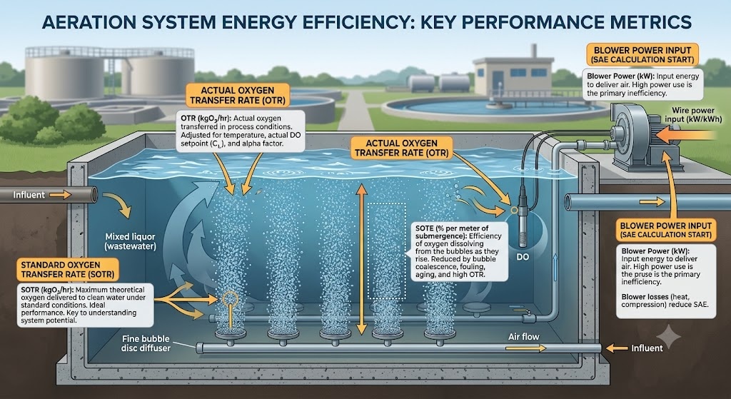
Before auditing anything, you need to speak the same language as your equipment. Four metrics define aeration system performance:
SOTR — Standard Oxygen Transfer Rate
The mass of oxygen transferred per hour under standard conditions (clean water, 20°C, zero DO, sea level). Units: kgO₂/hr. This is the manufacturer’s laboratory rating for a diffuser or aerator.
SOTE — Standard Oxygen Transfer Efficiency
The fraction of oxygen in the supplied air that actually dissolves into the water, under standard conditions. Expressed as % per meter of submergence or as total % for the system.
SOTE (%) = (O₂ dissolved / O₂ supplied) x 100
Fine bubble disc diffusers: 6–8% SOTE per meter of submergence
Coarse bubble diffusers: 3–4% SOTE per meter
Surface mechanical aerators: not depth-dependent; expressed as total SOTE
OTR — Actual (Field) Oxygen Transfer Rate
SOTR corrected for real process conditions — wastewater temperature, actual DO concentration, and alpha factor. This is what your diffusers actually deliver in the tank.
OTR = SOTR x alpha x (beta x C_s,T - C_L) / C_s,20 x theta^(T-20)
where:
SAE — Standard Aeration Efficiency
The single most useful number for an energy audit. SAE combines oxygen transfer and energy consumption into one comparable metric.
SAE (kgO₂/kWh) = SOTR (kgO₂/hr) / Wire power input to blower (kW)
The inverse — kWh/kgO₂ — is equally valid and more intuitive for cost calculation:
Specific energy (kWh/kgO₂) = 1 / SAE
SAE benchmarks by technology:
| Aeration technology | SAE (kgO₂/kWh) | Specific energy (kWh/kgO₂) |
|---|---|---|
| Fine bubble disc/tube/plate diffuser (optimized) | 2.5–5.0 | 0.20–0.40 |
| Fine bubble disc diffuser (typical operation) | 1.8–3.5 | 0.29–0.56 |
| Coarse bubble diffuser | 1.2–2.0 | 0.50–0.83 |
| Surface mechanical aerator (low-speed) | 1.2–2.5 | 0.40–0.83 |
| Surface mechanical aerator (high-speed) | 0.8–1.5 | 0.67–1.25 |
| Jet aerator | 1.0–2.0 | 0.50–1.00 |
| Deep shaft aeration (>15 m) | 3.5–6.0 | 0.17–0.29 |
If your plant’s calculated SAE is below 1.8 kgO₂/kWh for a fine bubble system, you have a recoverable performance problem — likely fouled diffusers, over-aeration, or inefficient blower operation.
You cannot audit what you haven’t measured. Most plants can calculate a rough SAE from existing instrumentation without any specialized testing equipment.
What you need:
Estimate daily oxygen demand (AOR — Actual Oxygen Requirement):
AOR (kgO₂/day) = (BOD removal oxygen demand) + (nitrification oxygen demand) - (denitrification credit)
BOD removal: ~1.0–1.2 kgO₂ per kg BOD removed (1.0 for simple BOD removal; 1.2 for combined BOD + nitrification systems)
Nitrification: 4.57 kgO₂ per kg NH₄-N oxidized
Denitrification credit: 2.86 kgO₂ recovered per kg NO₃-N reduced (if anoxic zones are present, subtract this)
Example — 10,000 m³/day municipal plant:
Calculate field SAE:
Convert to SOTR for clean-water equivalent comparison:
SOTR = AOR / (alpha × correction factor) ≈ AOR / (0.6 × 0.5) = AOR / 0.30
SOTR = 138 / 0.30 = 460 kgO₂/hr
Standard SAE = 460 / 191 = 2.41 kgO₂/kWh
This is near the lower end of the acceptable range for fine bubble systems — worth investigating.
Off-gas testing measures SOTE directly in process conditions by capturing the gas leaving the water surface in a floating hood and analyzing its oxygen content. This is the most accurate method for determining actual diffuser performance.
Equipment needed: floating gas collection hood, gas analyzer (O₂ and CO₂), airflow meter at blower.
SOTE (%) = (O₂ in - O₂ out) / O₂ in × 100
where O₂ in = airflow × 0.2095 (O₂ fraction of air) and O₂ out = O₂ concentration measured in collected off-gas × total off-gas flow rate.
Off-gas testing is the gold standard for post-cleaning or post-retrofit validation — it directly shows whether diffuser maintenance or replacement has improved performance. It requires specialized equipment and is typically conducted by a specialist team.
Blower efficiency determines how much of the electrical energy actually reaches the air stream. A blower delivering 85% of its rated output due to age, inlet filter fouling, or part-load operation wastes the rest as heat.
Isothermal power equation for blower efficiency assessment:
Theoretical isothermal power (kW) = Q_air × P_inlet × ln(P_outlet / P_inlet) / efficiency
where:
Blower efficiency benchmarks:
| Blower type | Peak isentropic efficiency | Typical field efficiency | Part-load efficiency (50% flow) |
|---|---|---|---|
| Roots tri-lobe (no VFD) | 55–65% | 50–60% | 35–45% |
| Roots tri-lobe (with VFD) | 55–65% | 55–62% | 50–58% |
| Rotary screw (with VFD) | 65–75% | 62–70% | 60–68% |
| Multi-stage centrifugal | 65–72% | 60–68% | 45–55% (surge risk) |
| High-speed turbo (direct drive) | 72–82% | 70–78% | 65–75% |
The most common efficiency problem in the field: blowers running at 40–60% of design flow continuously because the aeration system was designed for peak flow conditions that rarely occur. At 50% flow, a roots blower loses 15–25 percentage points of efficiency compared to its peak — wasting a significant fraction of every kWh consumed.
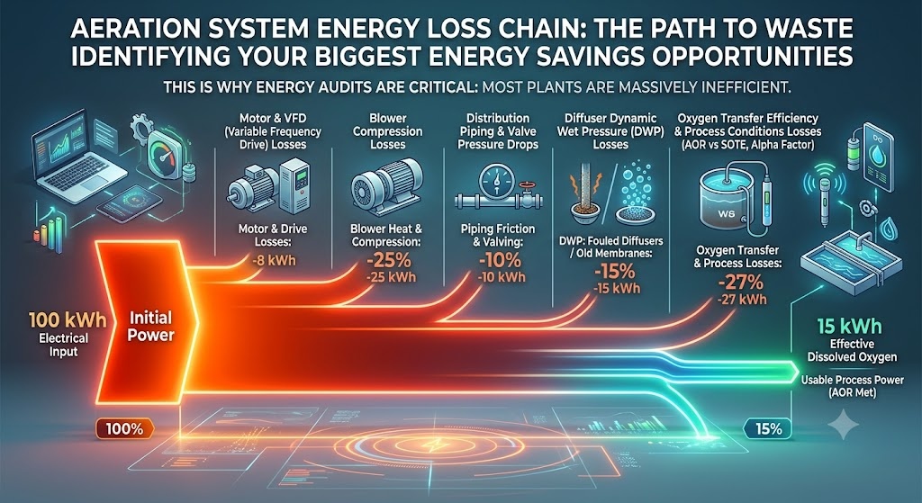
Every aeration system has four places where energy is lost between the electrical meter and the dissolved oxygen in the tank. Quantifying each loss identifies where to intervene.
The energy loss chain:
Electrical input → Blower motor losses → Blower compression losses → Pipe/valve distribution losses → Diffuser DWP losses → Oxygen transfer losses
| Loss stage | Typical magnitude | Cause | Audit check |
|---|---|---|---|
| Motor electrical losses | 3–8% | Motor ageing, partial load | Measure motor power factor and current draw |
| Blower compression losses | 20–35% | Blower type, operating point | Compare actual vs. theoretical isothermal power |
| Pipe and valve losses | 5–15% | Undersized pipe, fouled valves, excess control valves | Pressure drop across distribution system |
| Diffuser DWP losses | 5–25% | Fouling, ageing, over/under-flux | DWP measurement (see DWP article) |
| Oxygen transfer losses | 30–60% | Alpha factor, DO setpoint, bubble size | Off-gas test or SOTE estimation |
The combined effect: for every 100 kWh consumed by the blower motor, typically only 15–35 kWh ends up as dissolved oxygen in the mixed liquor.
Most plants were designed for peak daily/seasonal loads. Actual average load is typically 40–70% of peak. A blower running at fixed speed to meet peak demand runs at inefficient part load for most of its operating life.
Variable Frequency Drives (VFDs) allow blower speed to track actual oxygen demand. Tri-lobe positive displacement blowers with VFD for speed control offer a turndown of 60–70%, which allows great operational flexibility.
Energy savings from VFD: 15–30% of blower energy at typical plants. Payback: 2–4 years depending on electricity tariff and load variation.
VFD is most effective when: load varies significantly (diurnal variation > 2:1), multiple blowers are installed, current blowers run at >70% speed continuously.
VFD is least effective when: blowers already run at 95–100% speed most of the time (capacity-constrained plant), or when a roots blower is already throttled to minimum.
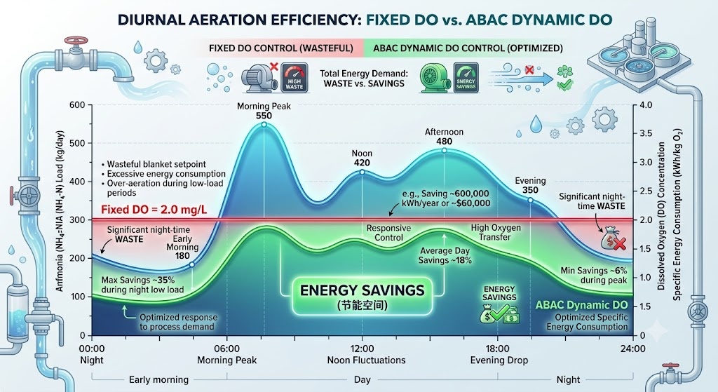
Most plants operate at a DO setpoint of 2.0 mg/L throughout the aeration basin — a blanket number that covers worst-case conditions. At average load conditions, this means chronic over-aeration.
Reducing the DO setpoint from 2.0 mg/L to 1.5 mg/L (still fully sufficient for nitrification at normal temperatures) typically reduces air demand by 10–20%. This is the lowest-cost intervention available — often achievable by reprogramming the PLC without any capital expenditure.
Important: DO setpoint reduction must be coupled with reliable DO sensor calibration. Drift in DO sensors is common and causes actual DO to be lower than the displayed value — reducing setpoint without recalibrating sensors risks process upset.
Standard DO control maintains a fixed DO concentration regardless of actual biological demand. ABAC goes one level deeper — it measures effluent ammonia concentration and adjusts the DO setpoint dynamically based on whether nitrification is complete.
Because OTE improves at lower DO concentrations, there are energy savings available by maintaining the minimum DO concentration that meets process objectives. ABAC systems take advantage of the influence of DO on both OTE and the rate of biological conversion of ammonia.
In practice: at night when ammonia load is low, ABAC allows DO to drop to 0.8–1.2 mg/L and still achieve full nitrification. During morning peak load, it increases DO to 2.5–3.0 mg/L before ammonia breaks through. This dynamic response is impossible with a fixed DO setpoint.
A case study published by Envirosim demonstrated that at a nitrifying activated sludge plant, manual DO control resulted in DO swings from 0.5 to 3.5 mg/L and 590 kWh/MGD blower energy. Conventional DO control reduced this by only 3%. ABAC reduced energy demand significantly further by narrowing the DO operating range to the minimum required for complete nitrification at all loading conditions.
Advanced control technologies including MPC integrated with AI and machine learning can decrease energy usage by 30–40% and enhance DO levels by 35–40% compared to manual operation.
ABAC implementation requirements: ammonia sensor (ion selective electrode or online analyzer) near effluent end of aeration basin; DO sensors in each control zone; SCADA integration; VFD blowers for response capability.
Fouled diffusers produce larger bubbles with lower SOTE, and raise DWP — meaning the blower must work harder to push the same air through. The combined effect of fouled diffusers at DWP = 100 mbar vs DWP = 20 mbar is a 15–25% increase in energy per unit of oxygen transferred.
The implementation of a properly designed aeration control system has been reported by the United States Environmental Protection Agency to reduce aeration energy by 25 to 40 percent. But this savings is only achievable when diffusers are clean — a fouled diffuser system negates the benefits of advanced control.
Diffuser maintenance priority order:
See the DWP article for full maintenance decision framework.
If the plant was built with roots tri-lobe blowers operating above 0.5 bar back-pressure — as many plants are, since roots blowers were the default technology for decades — replacing them with high-speed turbo blowers or rotary screw blowers delivers significant efficiency gains.
| Blower upgrade | Peak efficiency gain | Energy savings (indicative) | Payback |
|---|---|---|---|
| Roots → Rotary screw (same pressure) | +10–15 percentage points | 15–20% | 4–7 years |
| Roots → High-speed turbo | +15–25 percentage points | 20–30% | 5–9 years |
| Multi-stage centrifugal → Turbo | +8–15 percentage points | 10–20% | 5–8 years |
| Add VFD to existing screw blower | +8–15% at part load | 10–20% | 2–4 years |
Blower replacement is the highest capital cost intervention but delivers the most durable savings — efficiency gains are independent of operator behavior and do not degrade without major mechanical failure.
A complete aeration energy audit delivers a savings matrix: each opportunity quantified in kWh/year and $/year, with estimated implementation cost and simple payback period.
Example audit output — 10,000 m³/day municipal plant, 191 kW blower load, $0.10/kWh electricity:
| Opportunity | Energy saving | Annual saving | Implementation cost | Simple payback |
|---|---|---|---|---|
| DO setpoint 2.0 → 1.5 mg/L (PLC reprogramming) | 15% | $25,000 | $2,000 | 1 month |
| Diffuser burst cleaning + acid clean | 12% | $20,000 | $5,000 | 3 months |
| VFD on lead blower | 18% | $30,000 | $40,000 | 16 months |
| ABAC implementation | 20% | $33,000 | $80,000 | 29 months |
| Blower replacement (roots → turbo) | 25% | $42,000 | $250,000 | 71 months |
Note: savings are not fully additive — DO setpoint reduction and ABAC address overlapping issues. Combined realistic saving from all five measures: 35–50% of baseline aeration energy, with most of the saving achievable within 3 years through the first three measures alone.
Small WWTPs benefit from on/off and PID control methods, resulting in 10–25% energy savings and DO level reductions of 5–30%. Cascade control and model predictive control improve energy efficiency by 15–30% in medium-sized WWTPs. Advanced WWTPs utilizing MPC integrated with AI and machine learning can decrease energy usage by 30–40%.
| Plant size | Appropriate control strategy | Realistic energy saving |
|---|---|---|
| < 1,000 m³/day | On/off blower + manual DO adjustment | 5–15% |
| 1,000–5,000 m³/day | PID DO control + VFD | 15–25% |
| 5,000–20,000 m³/day | Cascade DO control + ABAC + VFD | 20–35% |
| > 20,000 m³/day | MPC + ABAC + multi-blower coordination | 25–40% |
| > 50,000 m³/day | MPC + AI/ML load prediction + full instrumentation | 30–45% |
One of the most frequently overlooked energy savings in plants with anoxic zones. During denitrification, bacteria use NO₃ as an electron acceptor instead of O₂ — effectively recovering oxygen from the nitrate molecule.
Oxygen credit = 2.86 kgO₂ per kg NO₃-N reduced
For a plant denitrifying 15 mg/L NO₃ from 10,000 m³/day flow:
At SAE = 2.5 kgO₂/kWh, this credit is worth: 429 / 2.5 = 172 kWh/day = $6,200/year
Plants that have anoxic zones but don’t account for the denitrification credit in their blower control logic are over-aerating and wasting energy equivalent to this credit every day.
Run this checklist before commissioning a full audit — it identifies the three most common quick wins:
1. Read blower discharge pressure and calculate DWP
2. Check blower operating point vs. design curve
3. Read average DO from SCADA trending (past 7 days)
4. Compare actual blower power to theoretical requirement
5. Check diurnal variation in blower output
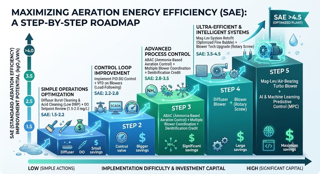
| Current SAE | Priority action | Expected SAE after action |
|---|---|---|
| < 1.5 kgO₂/kWh | Diffuser cleaning + DO setpoint review | 1.8–2.2 |
| 1.5–2.0 kgO₂/kWh | Add VFD + DO control | 2.2–2.8 |
| 2.0–2.5 kgO₂/kWh | Add ABAC + optimize diffuser coverage | 2.5–3.5 |
| 2.5–3.5 kgO₂/kWh | Blower technology upgrade if >10 yr old | 3.5–4.5 |
| > 3.5 kgO₂/kWh | Well-optimized — focus on diffuser maintenance | Maintain |
Related products: Nihao’s fine bubble disc diffusers, plate diffusers, tube diffusers, and aeration hose all support the diffuser-side optimizations described in this audit framework. Maintaining low DWP through EPDM or silicone membrane selection and regular cleaning is the highest-ROI, lowest-capital intervention available to most plant operators. Contact [email protected] for diffuser system assessment support.

86-15267462807


86-15267462807
